Plants and climate
To obtain palaeoclimate information from plant fossils two quite distinct approaches can be used. The first is taxon-based and relies on identifying fossils in terms of their nearest living relatives (NLRs) and is known as the NLR approach. Assuming this is done reliably the environmental regime under which the ancient plants once lived is derived from that tolerated today by the NLRs.
The second approach to obtaining palaeoclimate data using plants as a proxy is essentially ‘taxon-free’ in that no identification of the plant fossil is required. Instead, environmental data are obtained from plant form (physiognomy). This is the physiognomic approach.
“The present is the key to the past”
This idea, known to geologists as the principle of uniformitarianism, is generally thought to have been introduced through the writings of James Hutton in his Theory of the Earth (1795). William Whewell in 1832 coined the term ‘uniformitarianism’ as a foil to the then idea that Earth history revolves around a succession of catastrophies (catastrophism), but it was enshrined as a core idea of geology by Charles Lyell in his Principles of Geology (1830-33). However using this principle to interpret plant fossils in terms of climate has a far longer history.
In 1086 the Chinese writer Shen Kuo reasoned in a work called ‘Dream Pool Essays’ that because a certain kind of fossil was found in an area where the nearest living relative of that fossil no longer lives it follows that the climate must have changed since the time that the fossil was alive (Needham, 1986). This is remarkable not only for its use of uniformitarian thinking some seven hundred years before Hutton, but also because Shen Kuo recognised that fossils represent once living organisms and that climate is a key determinant as to where species can grow.
However, in order for this thinking to form the basis of a successful proxy for palaeoclimate the fossil has to be correctly identified, and it has to have a nearest living relative. For long extinct groups of plants this represents a problem that limits the use of NLR proxies in the deep past. In fact there is a high likelihood that Shen Kuo misidentified the Carboniferous Calamites (a relative of modern Equisetum, or mares tail) for bamboo (Fig. 1).
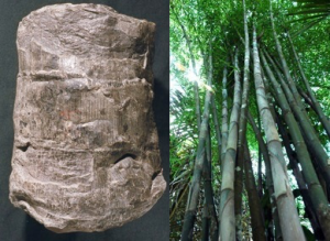
Figure 1. Left Calamites, Right, bamboo.
Ideally the NLR should be at the species level, but because species rarely survive unchanged for more than a million years or so often we have to make do with the genus level or, in extreme cases family level. Of course the more distant the relationship the more likely the fossil and living plant will have different climatic tolerance envelopes.
This brings us to evolution. Plants have to be well adapted to their local prevailing climate, including its extremes, or they will die. Evolution is all about adaptation brought about by random genetic change filtered by natural selection, so we would expect plants to change their climate tolerances over time. Such changes may not be apparent in the fossil record, particularly when overall plant form is rarely preserved in the fossil record; plants usually are preserved as isolated detached organs (leaves, pollen, wood etc., Fig. 2), not complete entities.
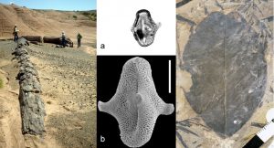
Figure. 2. The most common plant fossil parts are wood, pollen/spores and leaves. a) late Cretaceous fossil pollen Aquilapollenites mtchedlishvili Srivastava as seen in the light microscope and b) as seen using a scanning electron microscope. Scale bar = 10µm.
Potentially evolutionary change undermines the NLR approach but the effect can be minimised if we use several NLRs simultaneously. The more taxa are used in the analysis the more likely that anomalies due to evolutionary change in one or two taxa will be identified and can excluded from influencing the climate estimate. The Co-existence Approach (Mosbrugger and Utescher, 1997) and Bioclimatic Analysis (Greenwood et al., 2003; 2005) are two examples of such a multi-taxon approach. The main advantage of NLR proxies over other ways of determining past climate from plants is that they can be applied to any identifiable plant part such as pollen, wood, leaves, seeds and fruits. For two contrasting views of the issues associated with such approaches see Grimm and Denk (2012) and Utescher et al. (2014).
Further Reading:
- Greenwood, D.R., Moss, P., Rowett, A., Vadala, A. & Keefe, R. (2003) Plant communities and climate change in southeastern Australia during the early Paleogene. Geological Society of America Special Paper 369, 365–380.
- Greenwood, D.R., Archibald, S.B., Mathewes, R.W. & Moss, P.T. (2005) Fossil biotas from the Okanagan Highlands, southern British Columbia and northeastern Washington State: climates and ecosystems across an Eocene landscape. Canadian Journal of Earth Sciences 42, 167–185.
- Grimm, G.W. & Denk, T. (2012) Reliability and resolution of the coexistence approach — a revalidation using modern-day data. Review of Palaeobotany and Palynology 172, 33–47.
- Mosbrugger, V. & Utescher, T. (1997) The coexistence approach — a method for quantitative reconstructions of Tertiary terrestrial palaeoclimate data using plant fossils. Palaeogeography, Palaeoclimatology, Palaeoecology 134, 61–86.
- Needham, J. (1986) Science and Civilization in China: Volume 3, Mathematics and the Sciences of the Heavens and the Earth. Caves Books Ltd., Taipei.
- Utescher, T., Bruch, A.A., Erdei, B., François, L., Ivanov, D., Jacques, F.M.B., Kern, A.K., Liu, Y-S.(C)., Mosbrugger, V. & Spicer, R.A. (2014) The Coexistence Approach—Theoretical background and practical considerations of using plant fossils for climate quantification. Palaeogeography, Palaeoclimatology, Palaeoecology 410, 58–73.
Leaves and climate
An alternative, but complementary, way of using fossil plant fossils to quantify past climate is called the physiognomic approach. This relies on the adaptive relationship between plant morphology and climate. One common well-known physiognomic proxy is tree ring analysis where variations in wood cell form records changes in growing conditions and, because each wood cell takes only a few days to form, this gives a detailed record not just of climate (30 year average conditions) but almost day-to-day weather. Here though we are going to concentrate on the climate signal captured in the morphology of leaves.

Leaves have an intimate relationship with the atmosphere. After all, their primary function, photosynthesis, involves constantly processing the atmosphere, taking in carbon dioxide and giving out oxygen and water vapour. To conduct photosynthesis efficiently leaves have to be well adapted to their surrounding so that they can absorb as much light as possible, which requires them to be large as possible, but without investing too many resources, overheating or loosing too much water. They do, however, have to keep some water flowing through the plant from the roots to the leaves and then to the atmosphere in order to keep nutrients circulating in the plant body. When the air becomes saturated with water they have to pump water from the leaves, usually through glands on the leaf margins situated at the tips of ‘teeth’ (Fig. 3).
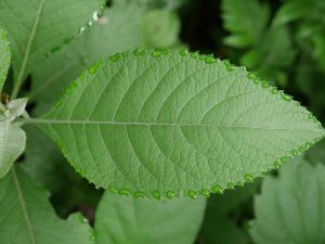
Figure 3. An example of guttation where a plant in a water-saturated atmosphere (often in the morning) pumps water out through marginal teeth to maintain water flow in the plant.
It is no surprise then that leaf form reflects the climate immediately surrounding the host plant. Leaf form tends to be optimised for efficient functioning under local conditions, and one reason why flowering plants are so successful is that they have the ability to produce many different leaf forms on an individual plant (i.e. from the same genome).
That plant growth forms and climate are related has been recognised since the writings of Theophrastus (around 300 BC) (Hort, 1948) and over the past 200 years or so has been commented upon frequently (e.g. Witham 1833; von Humbolt 1850; Seward 1892; Raunkiaer 1934; Givnish 1987). In the early 20th Century the relationship between the proportion of species with marginal teeth at any given location and mean annual temperature was noted (Bailey and Sinnott, 1915; 1916) and developed further some 60 years or so later (Wolfe, 1979).
However, we now know that through highly flexible yet integrated developmental pathways and pleiotropy (the production by a single gene of multiple features) (Schlichting 1989; Falconer & Mackay 1996; Juenger et al. 2005; Rodriguez et al. 2014) that leaves operate as complex systems where all features are linked to one another – no single feature has a simple relationship with a single climate variable. A change in one feature necessarily means a change in others if the leaf is to remain functionally efficient. At the macro scale this complex web of interrelationships is captured in Figure 4, but similarly the number and type of stomata are linked to vein architecture (Brodribb and Jordan, 2012), which is in turn linked to overall leaf form. This complex interaction of leaf characters and climate means that single character to single climate variable links must be spurious and unreliable (Yang et al., 2015).
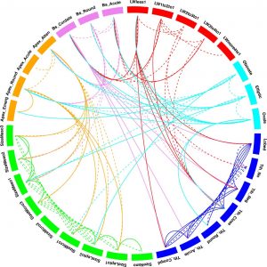
Fig. 4 Linkage diagram illustrating the relationships between leaf characters shown by the pairwise Pearson correlation coefficients. The 31 leaf characters (shown in summary form in Fig. 2) are grouped: lobing and tooth form, leaf size, apex form, base form, length-to-width ratio and shape. Leaf character groups are indicated by different colours: red – length-to-width ratios, light blue – leaf shape, dark blue – margin characters, green – leaf size, orange – apex characters, pink – base characters. The solid lines represent values of Pairwise Pearson correlation above a ≤ 0.5 (a significant positive correlation), while the dashed lines indicate correlations a ≥ -0.5 (a significant negative correlation). Some correlations are trivial in that they arise from the scoring regime (e.g., “no teeth” is negatively correlated with all tooth characters because leaves without teeth will not be scored for tooth characters) and are shown as links within leaf character groups. Meaningful correlations are those that link different character groups. For example the cordate base condition is positively correlated with several tooth characters. From Yang et al., (2015).
If numerous leaf features are linked to numerous climatic parameters the only way we can look at these relationships is by using multivariate statistical methods. The best known and most widely used such approach is called CLAMP – Climate Leaf Analysis Multivariate Program. This technique, in it most often used form, quantifies the combined relationships of 31 leaf form character states (Fig. 5) and 11 climate variables in patches of vegetation where there are at least 20 species of woody dicot flowering plants. For a more complete explanation of the technique please see the CLAMP website: http://clamp.ibcas.ac.cn.
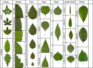
Figure 5. Summary of the leaf characters used in a CLAMP analysis. For the scoring protocols see the CLAMP website http://clamp.ibcas.ac.cn
One advantage of the CLAMP technique is that no leaf identification is required – it is a ‘taxon-free’ method. A disadvantage is that it can only be used on leaves of woody dicotyledonous flowering plants, which are not as commonly preserved as pollen.
Further Reading:
- Bailey, I.W., Sinnott, E.W. (1915) A botanical index of Cretaceous and Tertiary climates. Science 41, 831–834.
- Bailey, I.W., Sinnott, E.W. (1916) The climatic distribution of certain types of angiosperm leaves. Am. J. Bot. 3, 24–39.
- Brodribb, T.J., Jordan, G.J. (2012) Water supply and demand remain balanced during leaf acclimation of Nothofagus cunninghamii trees. New Phytologist 192, 437–448.
- Falconer, D.S. & Mackay, T.F.C. (1996) Introduction to quantitative genetics. Addison Wesley Longman, Harlow.
- Givnish, T.J. (1987) Comparative studies of leaf form: Assessing the relative roles of selective pressures and phylogenetic constraints. New Phytologist 106, 131–160.
- Hort, A. (Translator) (1948) Enquiry into Plants Vol. 1 by Theophrastus. Harvard University Press, Cambridge, Mass.
- Juenger, T., Pérez-Pérez, J.M. & Micol, J.L. (2005) Quantitative trait loci mapping of floral and leaf morphology traits in Arabidopsis thaliana: evidence for modular genetic architecture. Evolution and Development 7, 259–271.
- Raunkiaer, C. (1934) The life forms of plants and statistical plant geography. Oxford University Press, Oxford.
- Rodriguez, R.E., Debernardi, J.M. & Palatnik, J.F. (2014) Morphogenesis of simple leaves: regulation of leaf size and shape. WIREs Developmental Biology 3, 41–57.
- Schlichting, C.D. (1989) Phenotypic integration and environmental change. BioScience 39, 460–464.
- Seward, A.C. (1892) Fossil Plants as Tests of Climate. C.J. Clay and Sons. Cambridge University Press, London.
- von Humboldt, A. (1850) Aspects of Nature in Different Lands and different Climates; with Scientific Elucidations. Lea & Blanchard, Philadelphia, Pennsylvania.
- Witham, W. (1833) The internal structure of fossil vegetables found in the Carboniferous and Oolitic deposits of Great Britain. Edinburgh.
- Wolfe, J.A. (1979) Temperature parameters of humid to mesic forests of eastern Asia and relation to forests of other regions of the Northern Hemisphere and Australasia. United States Geological Survey Professional Paper 1106, 1–37.
- Yang, J., Spicer, R.A., Spicer, T.E.V., Arens, N.C., Jacques, F.M.B., Su, T., Kennedy, E.M., Herman, A.B., Steart, D.C., Srivastava, G., Mehrotra, R.C., Valdes, P.J., Mehrotra, N.C., Zhou, Z.K. & Lai, J.S. (2015) Leaf Form-Climate Relationships on the Global Stage: An Ensemble of Characters. Global Ecology and Biogeography 10, 1113–1125
Plants and palaeoaltimetry

Lapse Rates:
The most widely used way of estimating surface height from plant fossils is to estimate mean annual temperature and then apply a suitable lapse rate (the rate at which temperature changes, usually declines, with increasing height above sea level). Although having a sound basis in physics, standard atmospheric lapse rates, measured in the free atmosphere, are difficult to relate to plants, which are attached to land surfaces and not suspended in columns of air. Meyer (1992) refers instead to a terrestrial lapse rate that is measured along a surface transect with both vertical and horizontal components, and is based upon temperatures measured in standard meteorological stations sited in clearings. Usually this empirical terrestrial lapse rate is less than the atmospheric lapse rate because of daytime heating of near-surface air along slopes. It is only the terrestrial lapse rate that is applicable to plants.
In theory then the difference in elevation (∆Z) between two locations, one high and one low may be derived from the difference in surface temperature (T) between two locations, using Equation 1:
![]() (Equation 1)
(Equation 1)
where ![]() and is the lapse rate. Provided the elevation of one site above sea level is known the elevation above sea level for the other site can be derived.
and is the lapse rate. Provided the elevation of one site above sea level is known the elevation above sea level for the other site can be derived.
Terrestrial lapse rates are affected by a variety of conditions, including the state of the atmosphere, moisture, albedo of the ground surface, local and regional topography, time of day, season and the nature and source of predominant air masses. As such at any one location the terrestrial lapse rate cannot be assumed to be a uniform gradient. It can be highly variable in both time and space due to changing meteorological conditions, the composition of the atmosphere (including moisture content) and the dynamics of adiabatic processes.
Elevation itself is another factor. Because the ground surface is the primary source of atmospheric heating, the altitude of that surface has a large influence on the regional relationship between altitude and temperature. The classic example of this is the heating effect of the Tibetan Plateau where strong daytime warming of the near-surface air mass results in higher near-surface mean temperatures for the plateau surface than would occur in the free atmosphere at the same altitude in adjacent locations. This has long been regarded as a contributory factor in amplifying the Asian monsoon systems (e.g. Flohn 1968; Yanai & Wu 2006) although the overall effect of Tibet on the South Asian monsoon is more complex (Boos & Kuang 2010; Molnar et al. 2010).
Clearly there are major complications in the application of terrestrial lapse rates on mountain slopes, but perhaps the greatest issue affecting plant fossil assemblages is that they accumulate in topographic lows (e.g. inter-montane basins) and because night-time low temperatures are a component in the calculation of mean temperatures, inversions due to cold air drainage result in mean temperatures that are lower in many valleys and basins than would be expected. This often results in surface temperature rising, not cooling, with increasing elevation (Wolfe 1992).
Despite the many problems associated with using lapse rates they have the advantage that they can be used with any proxy that delivers temperature data, including those based on NLR or physiognomy.
Enthalpy and Moist Static Energy:
Using CLAMP it is possible to obtain a property of the atmosphere known as moist enthalpy and moist enthalpy can be used the determine the height above sea level that a leaf is or, in the case of a fossil, was growing (Forest et al., 1995). Based on the principle of conservation of energy the use of moist enthalpy for obtaining past surface heights is generally more reliable than using lapse rates.
Moist static energy (h) is the total specific energy content of air and is given by Equation 2,
![]() (Equation 2)
(Equation 2)
where c’p the specific heat capacity at a constant pressure of moist air, T is temperature (in K), Lv is latent heat of vapourization of water, q is specific humidity, g is acceleration due to gravity (a constant) and Z is elevation. This expression excludes kinetic energy but (except during hurricanes) this is very small (< 1%) in relation to the other terms. Compared to lapse rates moist static energy displays far less geographic variability. This is because it is very nearly constant and conserved along air parcel trajectories, being only changed by radiative heating and surface fluxes of latent and sensible heat. Moreover the value of h in the lower (sub-cloud) part of the atmosphere (< ~1.5 km above the earth’s surface and usually referred to as the boundary layer) is almost the same as the value of h in the upper troposphere because of convection (Betts 1982; Xu & Emanuel 1989). At mid latitudes large-scale tropospheric airflow moves from west to east and as a result contours of h are roughly aligned parallel to latitude and largely invariant with longitude (Forest et al. 1995).
Moist static energy is made up of two components: enthalpy and potential energy, as is shown in Equation 3,
![]() (Equation 3)
(Equation 3)
where H is enthalpy (c’pT + Lvq) and gZ is potential energy. As a parcel of air rises it gains potential energy and, because moist static energy remains the same, enthalpy decreases.
It follows, therefore, that because the value of h is conserved the difference in elevation between two locations at the same latitude is given by Equation 4:
![]() (Equation 4)
(Equation 4)
The simplicity of Equation 4, where the difference in enthalpy between two locations (Hlow-Hhigh) divided by the acceleration due to gravity (g) gives the elevation difference (∆Z) between those locations, offers a very attractive palaeoaltimeter for obtaining surface elevation above sea level (if Hlow is derived from a flora bounded by, or laterally equivalent to, marine units) or relative surface height differences (if the absolute elevation of both Hlow and Hhigh are unknown). Note that this simplicity only applies if Hlow and Hhigh are at the same latitude, or if latitudinal differences are known and can be corrected for.
For a recent example of the application of this technique see Ding et al. (2017).
Further Reading:
- Betts, A.K. (1982) Saturation point analysis of moist convective overturning. Journal of the Atmospheric Sciences 39, 1484–1505.
- Boos, W.R. & Kuang, Z. (2010) Dominant control of the South Asian monsoon by orographic insulation versus plateau heating. Nature 463, 218–222.
- Ding, L., Spicer, R.A., Yang, J., Xu, Q., Cai, F., Li, S., Lai, Q., Wang, H., Spicer, T.E.V., Yue, Y., Shukla, A., Srivastava, G., Khan, M.A., Bera, S., Mehrotra, R.C. (2017) Quantifying the rise of the Himalaya orogen and implications for the South Asian monsoon. Geology 45, 215–218.
- Flohn, H. (1968) Contributions to a meteorology of the Tibetan highlands. Atmospheric Science Paper 130, Department of Atmospheric Sciences, Colorado State University.
- Forest, C.E., Molnar, P. & Emanuel, K.E. (1995) Palaeoaltimetry from energy conservation principles. Nature 343, 249–253.
- Meyer, H.W. (1992) Lapse rates and other variables applied to estimating paleoaltitudes from fossil floras. Palaeogeography, Palaeoclimatology, Palaeoecology 99, 71–99.
- Molnar, P., Boos, W.R. & Battisti, D.S. (2010) Orographic controls on climate and paleoclimate of Asia: thermal and mechanical roles for the Tibetan Plateau. Annual Review of Earth and Planetary Sciences 38, 77–102.
- Wolfe, J.A. (1992) An analysis of present-day terrestrial lapse rates in the western conterminous United States and their significance to paleoaltitudinal estimates. United States Geological Survey Bulletin 1964, 1–35.
- Xu, K-M. & Emanuel, K.A. (1989) Is the tropical atmosphere conditionally unstable? Monthly Weather Review 117, 1471–1479.
- Yanai, M. & Wu, G.X. (2006) Effects of the Tibetan Plateau. In Wang, B. (ed) The Asian Monsoon. Berlin, Springer. pp. 513–49.
Plants and vegetation by Bob Spicer.
Biomarkers:
The leaf wax composition and stable carbon isotope value of conifers: should we care?
The stable carbon isotopic composition (δ13C) of organic matter provides key information about fundamental metabolic pathways used by the organism and the environmental conditions during formation. For example, trees in a temperate forest have a different isotopic composition compared to grasses on the African savannah and both have a very different isotopic composition compared to bacterial methane (Fig. 1). As such δ13C is a commonly used tool in organic geochemistry and has been applied to a wide-range of environmental and paleoclimatological problems.
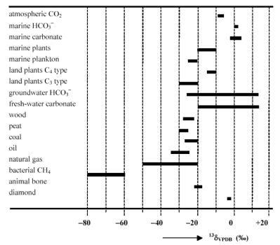 Fig. 1; Generalised overview of the stable carbon isotopic composition (δ13C) of a range of organic and inorganic material.

Introduction into stable carbon isotopes
Carbon, the fourth most abundant element in the universe, exists in two stable forms; 12C with a core consisting of 6 neutrons and 6 protons and 13C which has one additional neutron. Of all carbon on earth, 99% is present as 12C and 1% consists as 13C. In addition to these two stable forms, in nature a small fraction of carbon exists as 14C, which is radioactive and decays into 14N with a half-life of ~ 5,700 yrs. In material older than ~ 57,000 years normally all 14C has decayed into 14N and this material is defined as being “radiocarbon dead”.
The ratio of 13C compared to 12C is generally expressed as δ13C, which reflects the ratio of 13C/12C in a natural sample compared to an inorganic standard called the Vienna Pee Dee Belemnite (VPDB).

Organisms generally prefer 12C over 13C because it is a little bit lighter, leading to an enrichment of 12C over 13C in most types of organic matter. As VPDB is rich in 13C, most organic matter is depleted in 13C relative to the standard (Fig. 1). For example, if organic matter has a δ13C value of -25 ‰, this sample has 25 fewer 13C atoms per thousand carbon atoms compared to that of the inorganic standard and is depleted in 13C.
Bulk versus compound specific δ13C
Although bulk δ13C values indicate the fundamental metabolic pathways used by the organism and the environmental conditions during formation, in geological archives, such as sediments, bulk δ13C values are often not very diagnostic. This is because bulk δ13C reflects a mixture of different types of organic matter [Pagani et al. 2000]. As a result changes in the relative contribution of different types of organic matter can have a large impact on bulk δ13C values. To circumvent this complication, organic geochemists use combustion isotope ratio mass spectrometry coupled to gas chromatography to determine the δ13C of individual lipids. If diagnostic lipids are targeted (biomarkers), changes in compound specific δ13C values reflect changes in the δ13C of specific (parts of) organisms and are not thought to be biased by changes in the type of organic matter.
Compound specific δ13C
One of the most widely used biomarkers for paleoclimatological studies are higher plant waxes. These waxes consist of long-chain aliphatic compounds such as n-alkanes (Fig. 2) [Eglinton and Hamilton, 1967].
 Fig. 2: (L) pea leaf 5000x magnified, clearly showing the epicuticular waxes. (R) a wax-free beetroot leaf. Pictures from G. Eglinton.

Plants produce the epicuticular waxes to protect their leaves from the environment and to reduce water loss. Importantly, these biomarkers are easily transported by wind and rivers over thousand of kilometers [Simoneit, 1977], are very resistant to degradation and can be abundant in ancient open marine sediments [Schefuss et al., 2003; Naafs et al. 2012] making these ideal targets for compound specific δ13C studies. However, although most higher plants produce epicuticular waxes, there is a large spread in both their abundance and δ13C value because different higher plants use different metabolic pathways. One of the key differences is the mechanism used to fix carbon during photosynthesis (see below)
C3 and C4 plants
There are three distinct types of higher plants: C3 plants, C4 plants, and CAM plants. CAM plants, which use the crassulacean acid metabolism (CAM), form a minor component of high-plants (7% of total). As such, we will not discuss these in much detail today. The majority (85%) of higher plants are C3 plants. Most shrubs, herbs, trees, and cool-season grasses are C3 plants. In C3 plants CO2 is directly provided to Rubisco, the key-enzyme in the Calvin cycle (Fig. 3). The down-side of this mechanism is that oxygen can also bind to Rubisco in a process that is called photorespiration, which costs energy without fixing carbon. C4 plants differ from C3 plants in that CO2 is first concentrated in the mesophyll cell before it enters the Calvin cycle, ensuring that Rubisco is mainly used to fix carbon (Fig. 3). Typical C4 plants include tropical grasses and sedges and C4 plants are responsible for roughly a third of the global terrestrial carbon fixation. Because of their different pathways to fix carbon the organic matter of C3 and C4 plants, including the epicuticular waxes, have a distinctly different δ13C value. Specifically, C3 plants are generally ~ 10 ‰ lighter compared to C4 plants (Fig. 1).
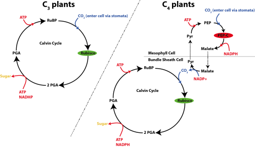 Fig. 3: Overview of carbon fixation pathway used by C3 (left) and C4 plants (right).

The paper (Diefendorf et al., 2015; Leaf wax composition and carbon isotopes vary among major conifer groups)
Conifers are an essential component of modern day ecosystems. They are particularly abundant within northern hemisphere high-elevation and high-latitude ecosystems but can also be found in tropical and southern hemisphere ecosystems. Previous studies (e.g. Diefendorf et al., 2011; Bush and McInerney, 2013) suggest that conifers do not produce large quantities of epicuticular plant waxes (e.g. n-alkanes) compared to angiosperm plants. This would suggest that conifers do not form a significant source of epicuticular plant waxes in geological archives such as marine sediments or lignite deposits. However these previous studies were based on a limited number of conifer species. For example, tropical and Southern Hemisphere conifer species had not been explicitly studied for their epicuticular plant waxes chemistry.
 Figure 4: Pictures of typical conifers: a) Cupressaceae; b) Taxaceae; c) Sciadopityaceae; d) Podocarpaceae; e) Araucariaceae; f) Pinaceae

In this paper Diefendorf et al. (2015) set out to fill the gap in our understanding of the contribution of conifer-derived plant waxes (predominantly n-alkanes) in natural archives. In total, 43 conifer species were sampled from the Botanical Garden at Berkley during December 2011. Sampling the conifers at the same location and the same time ensured that all plants experienced similar climatic variables and the only variable was plant species. Plant waxes were extracted from the powdered needles by means of solvent extraction and analyzed by means of GC-FID. The δ13C was determined by GC-C-IRMS.
Abundance and δ13C of n-alkanes in conifers
Previous studies (Diefendorf et al. 2011) have shown that the contribution of n-alkanes to the sedimentary pool is fairly insignificant compared to that of the angiosperm contribution (<200x higher). However, these new results indicate that conifers can be an important source of n-alkanes in natural archives. Their abundance in and on the needles of conifer trees rivals that of the angiosperms gram per gram.
Interestingly the concentration of n-alkanes is highly variable among different conifer groups (Fig. 5). In the early diverging taxodioid lineages, the concentrations of n-alkanes is low, while higher concentrations are found in other species. A particularly strong phylogenetic signal can be observed in the n-C29 alkane abundance and in the average chain length (ACL), complicating the use of ACL in natural archives to infer climatic changes.
 Figure 5: Abundance of n-alkanes on conifer trees with the evolution of the phylogenetic tree indicated beneath. Modified from Diefendorf et al. 2015

In this study the authors show that the overall fractionation between bulk conifer leaf and leaf waxes such as n-alkanes is around 4.1‰. This is consistent with previous studies and similar to that observed in angiosperms. There are however distinct differences in the fractionation of 13C across the different analyzed phylogenentic groups. For example Taxaceae is characterized by a particularly large fractionation of 8 ‰ (Diefendorf et al. 2015). The authors suggest that this is a result difference in the metabolic pathways associated with carbon fixation, but acknowledge that further research is required. The large difference in leaf/wax fractionation values observed in some conifer species may therefore complicate our understanding of sedimentary n-alkane δ13C records.
In summary, this paper indicates that conifers should be taken seriously in terms of their input into sedimentary systems. Their contribution to the n-alkane pool in natural archives cannot be neglected, specifically since this study has shown that the concentrations of n-alkanes in some conifers is significant even compared to that of angiosperms. In addition the authors stress the importance of taking conifers into account when interpreting δ13C-values from paleo-archives, because of the difference in fractionation between angiosperms and conifers.
Further reading:
- Bush and McInerney (2013) Leaf wax n-alkane distributions in and across modern plants: implications for paleoecology and chemotaxonomy. GCA. 117. 161-179.
- Diefendorf et al. (2011) Production of n-alkyl lipids in living plants and implications for the geologic past. GCA. 75. 7472-7485
- Diefendorf et al., (2015) Leaf wax composition and carbon isotopes vary among major conifer groups. GCA, 170, 145-156
- Eglinton and Hamilton (1967) Leaf epicuticular waxes. Science. 156. 1322-1335
- Naafs et al. (2012) Strengthening of North American dust sources during the late Pliocene (2.7 Ma). EPSL. 317-318.8-19
- Pagani et al. (2000) Isotope analyses of molecular and total organic carbon from Miocene sediments. GCA. 64. 37-49
- Schefuβ (2003) Carbon isotope analyses of n-alkanes in dust from the lower atmosphere over the central eastern Atlantic. GCA. 67. 1757-1767
- Simoneit (1977) Organic matter in Eolian dusts over the Atlantic Ocean. Marine Chemistry. 5. 443-464
By Jan Peter Mayser and Bristol University Organic Geochemistry Unit (OGU).

